Linear Regression for Marketing Analytics is one of the most powerful and basic concepts to get started in Marketing Analytics with. If you are looking to start off with learning Machine Learning which can lend a helping hand to your Marketing education then Linear Regression is the topic to get started with.
You as a marketer know that Machine Learning and Data Science have a significant impact on the decision making process in the field of Marketing. In the field of Marketing, Marketing Analytics helps in giving conclusive reasoning for most of the things, which for years and years has run on the golden gut of marketers.
Learning Regression for Marketing Analytics gives you the ability to predict various marketing variables which may or may not have any visible pattern to them. In this discussion, I will give you an introduction to what is linear regression and how it can transform your marketing and sales analytics.
Therefore, if you are willing to get started with Machine Learning or Marketing Analytics, Linear Regression is the place to begin. I assure you that after this discussion, Linear Regression, as a concept will be crystal clear to you.
Machine Learning for Marketing Analytics
You may already have the understanding of the fact that machine learning algorithms can be broadly divided into two categories: Supervised and Unsupervised Learning.
In Supervised Learning, the dataset that you would work with has the observed values from the past of the variable that you are looking to predict.
For example, you could be required to create a model for predicting the Sales of a product basis the Advertising Expenditure and Sales Expenditure for a given month.
You would begin by asking the Sales Manager for the data for the previous months, expecting that he would share with you a well laid out excel with Quarter, Advertising Expenditure, Sales Expenditure and the Sales for that quarter in different columns.
With such a dataset in your possession, the job of the predictive algorithm that you create will be to find the relationship between these variables. The relationship should be generalized enough so that when you enter the advertising and sales expenditures for the coming quarter, it can give the predicted sales for that quarter.
Unsupervised Learning is when this observed variable is not made available to you. In that case you will find yourself solving a different kind of marketing problem altogether and not that of prediction of a variable. Unsupervised Learning is not a part of this discussion.
Supervised Learning has two sub-categories of problem: Regression and Classification.
If you are pressed for time, you can go ahead and watch my video first in which I have explained all the concepts that I have shared below.
Supervised Learning for Marketing Analytics
I shared a common marketing use case above. In that example, you had to predict the sales for the quarter using two different kinds of expenditure variables. Now, we know that the value of sales can be any number - arguably a positive one. The sales could, therefore, range from anywhere between 0 to some really high number.
Such a variable is a continuous variable which can have any value in a really high range. And this, infact, is the simplest way to understand what regression is.
A prediction problem in which the variable to be predicted is a continuous variable is a Regression problem.
Let’s look at an entirely different marketing use case to understand what is not a regression problem.
You have been recruited in the marketing team of a large private bank (a common placement for many business students).
You are given the data of the bank’s list of prospects of the last year with details like Age, Job, Marital Status, No. of Children, Previous Loans, Previous Defaults etc. Along with that you are also provided with the information whether the person took the loan from the bank or not (0 for did not take the loan and 1 for did take the loan).
Your job as a young analytical marketer is to predict whether a prospect which comes in, in the future will take the loan from your bank or not.
Now, please note that in such a prediction problem your task is to just classify the prospects basis your algorithm’s understanding of whether the prospect will buy or not. Which means that the possible values for the outcome are discrete (0 or 1) and not continuous.
A prediction problem in which the variable to be predicted is a discrete variable is a Classification problem.
There are a variety of problems across industries that are prediction problems. My objective of this discussion is to equip you with the intuition and some hands-on coding of Linear Regression so that you can appreciate the use cases irrespective of the industry.
Vocabulary of Regression
Before I dive straight into what Linear Regression is, let me help you in forming an understanding of the vocabulary used when explaining regression. I will link it to the use cases mentioned above. So just reading through it will give you a complete understanding of what is what.
Target Variable: The variable to be predicted is called the Target Variable. When you had to predict the Sales for the quarter using the Advertising Expenditure and Sales Expenditure, the Sales is the target variable.
Naturally, the target variable can also be referred to as the Dependent Variable as its value is dependent on the other variables in the system. Even in our marketing use case, obviously, the Sales is dependent on how much expenditure you have done on Advertisements and on Sales Promotions.
The target variable is commonly denoted as y.
Feature Variable: All the other variables that are used to predict the target variable are called the Feature variables.
The feature variables can also be called Independent Variables. In the examples, the Advertising and Sales Promotion expenditures are the independent variables. Also, imagine that there is a different machine learning problem altogether of image recognition. In such a problem, each of the pixels is a feature variable.
The feature variable is commonly denoted as x. Multiple feature variables get denoted as x0, x1, x2,...., xn.
Finally, let me clarify to you as to what are the different names with which these two variables can be referred to.
- Independent Variable (x) and Dependent Variable (y)
- Feature Variable (x) and Target Variable (y)
- Predictor Variable (x) and Predicted Variable (y)
- Input Variable (x) and Output Variable (y)
Introduction to Linear Regression
There are many Regression Models out of which the most basic regression model is the Linear Regression. For Nonlinear Regression, there are different models like Generalized Additive Models (GAMS) and tree-based models which can be used for regression.
Since you are starting off with Marketing Analytics, my objective in this discussion is to take you only through Linear Regression for Marketing Analytics and develop your understanding with that as a base.
Note: What I am going to share with you in the remaining part of the article tends to tune out a lot of people who are frightened by anything that even looks like Math. You would see some mathematical equations with unique notations, and some formulas as well.
None of it is a mathematical concept which you would not have studied in school. If you just manage to sit through it, you will realize that it is nothing but plain English written in a jazzed up manner with equations, which by the way are equally important.
For you as an Analytical Marketer, the intuition is important so please just focus on that.
A linear regression model for a use case which has just one independent/feature variable would look like:

When you use more than one feature variable in your model then the linear regression model will look like:

Let me quickly decipher what this equation means.
What are the β Parameters?
The symbols that you see, β0, β1, β2, are called Model Parameters. These are constants which determine the predicted value of the target variable. These can also be referred to as Model Coefficients or Parameters.
Specifically, β0 is referred to as the Bias Parameter. You will notice that this is not multiplied with any variable/feature in the model and is a standalone parameter that adjusts the model.
Notice carefully that I referred to these Model Parameters (β) as Constants and the features (x) as Variables. This difference needs to be understood and proper usage of the terms makes a lot of difference in understanding the topic.
Why is the predicted variable ŷ and not y?
As I had mentioned above, y is the target variable, which is the variable we are trying to predict. Now, while y represents the actual value of the variable to be predicted, ŷ represents the predicted value of the variable.
Since, there is always some error in the prediction that is why the predicted value is represented with a different notation from the actual variable.
Why is this called a ‘Linear’ regression model?
This is a simple concept straight from your class 10th textbook. If you notice the equation again, you would see that each of the independent variables (x) appears with the power of 1 (degree 1). This means that the variables are not of a higher power (i.e. x2, x3 ..).
Such a model will always be represented by a straight line when plotted on a graph, as I would show in the later part of this discussion.
Visual Representation of Linear Regression
I briefly touched upon a use case above in which you were to predict the Sales or a quarter basis the Advertisement Expenditure and the Sales Expenditure. Since there are two features in this model, the structure of this model will be like the equation below:

However, for simplicity, let us assume that for the features the Sales Manager could only provide the data for the Advertisement Expenditure and, therefore, there will only be a single feature in our model. In this situation, this is how our model equation is going to look like.

Here is the exact data that you received from the sales manager for you to work on.
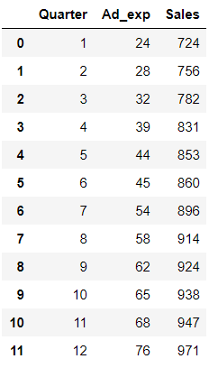
This data shows that for a Quarter 1, when the Advertisement Expenditure was 24,000, the sales were 724,000. I’m ignoring the units of currency for the time being. It could be Indian Rupee (INR) or United States Dollars (USD) or anything else.
Now, I went ahead and plotted both of these variables on a scatter plot with the Advertisement Expenditure on the x-axis and the Sales on the y-axis.
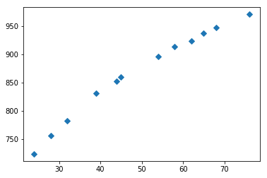
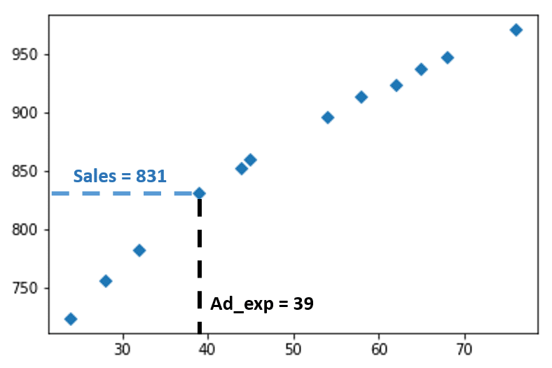
In this scatter plot, each dot represents one quarter given in the table. For that particular quarter, we will be able to determine the Advertisement Expenditure and the resulting Sales from the x and y axis, respectively.
How would you predict using Linear Regression?
You would remember that the objective for this exercise is to be able to predict the sales of the future quarters based on the features that we have. And in this case, we have just one feature variable, i.e. the Ad_Exp.
In order to know where the next dot will lie on the scatter plot you need to find the equation of a straight line which passes through these points hence representing a trend.
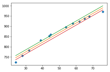
Now, through Python I have drawn three lines which pass through these plots. Each of these three lines are represented by three different equations. Just by looking at the three, you can say that the one in the middle seems to be passing through the points just ‘perfectly’. How do we determine whether this line passes through the points perfectly or not?.
Read on.
Which is the best trendline in Linear Regression?
Now obviously, you don’t need to make these three lines on your scatter plot every time you do linear regression. It is just for me to explain to you the intuition behind how we choose the best fitting linear line.
The best trendline which passes through the scatter plots is the one which minimizes the difference between the actual value and the predicted value across all the points.
If you magnify at one of the points you will see what exactly is this difference between the actual and the predicted value. A metric that is used to capture the error of the entire model across all the points is called Residual Sum of Squares (RSS) which will be discussed in my next article on errors.
But to explain briefly, each of these distances (of each of the points) from the best fitting line is squared and added. What we finally get is the Residual Sum of Squares.
As we had already understood from our intuition, out of the three lines that I had plotted, the one at the center seems to be the one with least difference across all the points. And if we run the curve fitting on Python, it indeed turns out to be the best fitting line for the scatter plot.
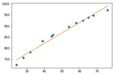
For this part of the discussion, my purpose was to just give you the intuition of Linear Regression for Marketing Analytics.
And with this you should be able to understand what is the objective of a linear regression problem. From what you have seen above, you can simply say that the objective of a linear regression problem is to determine the regression model parameters (β0, β1, β..) that minimize the error of the model.
Notice again, that this is a linear i.e. a straight line and it is not at all necessary that your trendline should be straight.
Non-linear regression is something that I will discuss later in the series once I have helped you develop an understanding for regression.
Hands-on Coding: Linear Regression Model with Marketing Data
This is the section where you will learn how to perform the regression in Python. Continuing with the same data that the Sales Manager had shared with you.

Sales is the target variable that needs to be predicted. Now, based on this data, your objective is to create a predictive model (just like the equation above), an equation in which you can plug in the Ad_exp value for a future quarter and predict the Sales for that quarter.
Let us straightaway get down to some hands-on coding to get this prediction done. Please do not feel left out if you do not have experience with Python. You will not require any pre-requisite knowledge. In fact the best way to learn is to get your hands dirty by solving a problem - like the one we are doing.
Step 1: Importing Python Libraries
The first step is to fire up your Jupyter notebook and load all the prerequisite libraries in your Jupyter notebook. Here are the important libraries that we will be needing for this linear regression.
- numpy (to perform certain mathematical operations for regression)
- pandas (the data that you load will be stored in a pandas DataFrames)
- matplotlib.pyplot (you will use matplotlib to plot the data)
In order to load these, just start with these few lines of codes in your first cell:
The last line of code helps in displaying all the graphs that we will be making within the Jupyter notebook.
Step 2: Loading the data in a DataFrame
Let me now import my data into a DataFrame. A DataFrame is a data type in Python. The simplest way to understand it would be that it stores all your data as a table. And it will be on this table where we will perform all of our Python operations.
Now, I am saving my table (which you saw above) in a variable called ‘data’. Further, after the equal to ‘=’ sign, I have used a command pd.read_csv.
This ensures that the .csv file which I have on my laptop at the file location mentioned in the path, gets loaded onto my Jupyter notebook. Please note that you will need to enter the path of the location where the .csv is stored in your laptop.
By running just the variable name ‘data’, as I have done in the second line of code, you will see the entire table loaded as a DataFrame.

Step 3: Separating the Feature and the Target Variable
You already know that the Ad_exp is the feature variable or the independent variable. Basis this variable, the target variable i.e. the Sales needs to be predicted.
Therefore, just like a classic mathematical equation, let me store the Ad_exp values in a variable x and the Sales values in a variable y. This notation also makes sense because in a mathematical equation y is the output variable and x is the input variable. Same is the case here.
The last line of code will display a scatter-plot on your Jupyter notebook which will look like this:

Please note, this is the same plot that you saw above in the intuition section.
Step 4: Machine Learning! Line fitting
Let me tell you that till now you have not done any machine learning. This was just some basic level data cleaning/data preparation.
The glamorous Machine Learning part of the code starts here and also ends with this one line of code.
From the Numpy library that you had installed, you will now be using the polyfit() method to find the coefficients of the linear line that fit the curve.
You already know from you school level math that the equation of a linear line is given by:
Y = mX + c
Here, the m is the slope of the line and c is the y-intercept. This trendline that we are trying to find here is no different. It follows the same equation and with this code we will be able to find the m and c values for it.
This method needs three parameters: the previously defined input and output variables (x, y) — and an integer, too: 1. This latter number defines the degree of the polynomial you want to fit.
You would have understood that if you changed that number from 1 to 2, 3, 4 and so on, it would become a higher degree of regression also referred to as Polynomial Regression.
That is also something that I will be discussing with you in the coming weeks.
But, as soon as you run this code, you see an output which is an array of two digits. These two digits are nothing but the values of m and c from the equation of a straight line.
Therefore, we now know that the best trendline that describes our data is:
y = 633.9931736 + (4.68585196 * x)
If you realize, we are actually done with our prediction problem. With this equation given above, you can just plug in the value of x, which you should remember is Advertising Expenditure, and you will get the value of y, i.e. the Sales that you are likely to make in that quarter.
But, since we are already doing some interesting stuff in python here, why do we have to manually find the value of Sales. Let’s make this better in our last and final step.
Step 5: Making the Predictions
Instead of doing the calculations manually in that equation, you can use another method that is made possible with the Numpy library that we had imported. The method is called poly1d()
Please follow the code given below.
We had stored the values of our equation coefficients in ‘model’. I created a variable Predict which now carried all this model data and also had the ability to predict value courtesy the Numpy method poly1d().
Now, when I entered Ad_Expenditure as 51, you saw that the predicted sales for it is shown to be 872.971.
Congratulations on your first step towards Marketing Analytics!
By executing these simple lines of code, you have successfully taken the first step towards learning Marketing Analytics. This is big!
Let me tell you that Linear Regression is a fundamental concept in Marketing Analytics and in Data Science in general. Therefore, you should definitely spend all that time that you need to understand it really well.
Things get interesting from here. I have not yet spoken about how to measure the accuracy of your system. I have also not mentioned how to perform this regression if there were more than one feature or independent variable. That is called Multiple Regression.
Gradually as we proceed in this journey, I will take you through all of these concepts and also through higher order regression i.e. the polynomial regression.
Conclusion
Having covered the most fundamental concept in machine learning, you are now ready to implement it on some of your datasets.
Whatever you learned in this discussion is more than sufficient for you to pick a simple dataset from your work and go ahead to create a linear regression model on it.
If you are not able to find a dataset for practice, stay rest assured. You can download a practice dataset for Linear Regression. This is a toy dataset that I have created for you practice so that you can get the necessary confidence.
Further, if you want to speed up the process of learning Marketing Analytics you can consider taking up this Data Scientist with Python career track on DataCamp. In order to help you get started with the career track, I have crafted a study plan for you so that you can sail through the course with ease.
The form you have selected does not exist.
Let’s learn some more Marketing Analytics in our next discussion.






Darpan thank you for thorough explanation, it’s very useful.
I have come across data where some sales values are negative, and advertising expenditure much higher than sales in general (to the effect of 100x). What would be the best approach in dealing with negative values? Thank you.